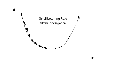
 (Fig. 1a)
 (Fig. 1a)
Recall that gradient descent requires a reasonable learning rate to work well: if it is too low (Fig. 1a), convergence will be very slow; set it too high, and the network will diverge (Fig. 1b).
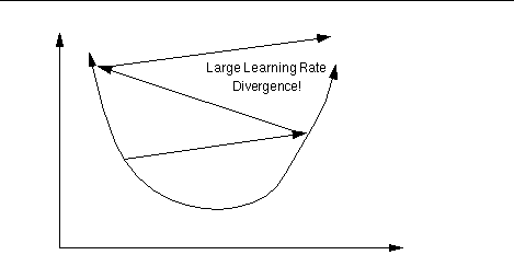 (Fig. 1b)
Unfortunately the best learning rate is typically different for each weight in the network! Sometimes these differences are small enough for a single, global compromise learning rate to work well - other times not. We call a network ill-conditioned if it requires learning rates for its weights that differ by so much that there is no global rate at which the network learns reasonably well. The error function for such a network is characterized by long, narrow valleys:
 (Fig. 2)
(Mathematically, ill-conditioning is characterized by a high condition number. The condition number is the ratio between the largest and the smallest eigenvalue of the network's Hessian. The Hessian is the matrix of second derivatives of the loss function with respect to the weights. Although it is possible to calculate the Hessian for a multi-layer network and determine its condition number explicitly, it is a rather complicated procedure, and rarely done.)
Ill-conditioning in neural networks can be caused by the training data, the network's architecture, and/or its initial weights. Typical problems are: having large inputs or target valuess, having both large and small layers in the network, having more than one hidden layer, and having initial weights that are too large or too small. This should make it clear that ill-conditioning is a very common problem indeed! In what follows, we look at each possible source of ill-conditioning, and describe a simple method to remove the problem. Since these methods are all used before training of the network begins, we refer to them as preconditioning techniques.
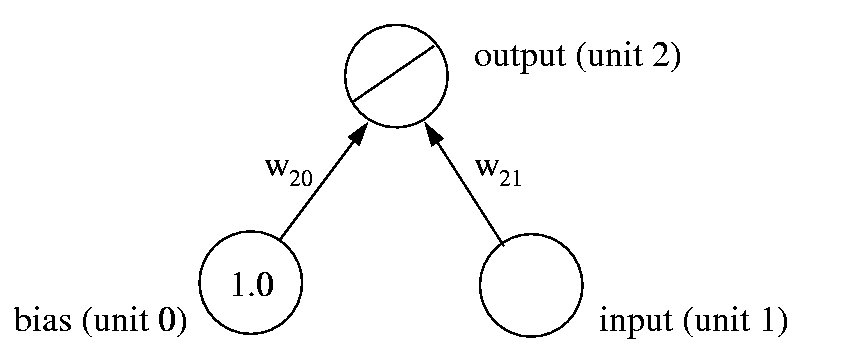 (Fig. 3)
Recall the simple linear network (Fig. 3) we first used to learn the car data set. When we presented the best linear fit, we had rescaled both the x (input) and y (target) axes. Why did we do this? Consider what would happen if we used the original data directly instead: the input (weight of the car) would be quite large - over 3000 (pounds) on average. To map such large inputs onto the far smaller targets, the weight from input to output must become quite small - about -0.01. Now assume that we are 10% (0.001) away from the optimal value. This would cause an error of (typically) 3000*0.001 = 3 at the output. At learning rate µ, the weight change resulting from this error would be µ*3*3000 = 9000 µ. For stable convergence, this should be smaller than the distances to the weight's optimal value: 9000 µ < 0.001, giving us µ < 10-7, a very small learning rate. (And this is for online learning - for batch learning, where the weight changes for several patterns are added up, the learning rate would have to be even smaller!)
Why should such a small learning rate be a problem? Consider that the bias unit has a constant output of 1. A bias weight that is, say, 0.1 away from its optimal value would therefore have a gradient of 0.1. At a learning rate of 10-7, however, it would take 10 million steps to move the bias weight by this distance! This is a clear case of ill-conditioning caused by the vastly different scale of input and bias values. The solution is simple: normalize the input, so that it has an average of zero and a standard deviation of one. Normalization is a two-step process:
| To normalize a variable, first |
|
Note that for our purposes it is not really necessary to calculate the mean and standard deviation of each input exactly - approximate values are perfectly sufficient. (In the case of the car data, the "mean" of 3000 and "standard deviation" of 1000 were simply guessed after looking at the data plot.) This means that in situations where the training data is not known in advance, estimates based on either prior knowledge or a small sample of the data are usually good enough. If the data is a time series x(t), you may also want to consider using the first differences x(t) - x(t-1) as network inputs instead; they have zero mean as long as x(t) is stationary. Whichever way you do it, remember that you should always
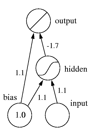
| (Fig. 4) |
To see why the target values should also be normalized, consider the network we've used to fit a sigmoid to the car data (Fig. 4). If the target values were those found in the original data, the weight from hidden to output unit would have to be 10 times larger. The error signal propagated back to the hidden unit would thus be multiplied by 17 along the way. In order to compensate for this, the global learning rate would have to be lowered correspondingly, slowing down the weights that go directly to the output unit. Thus while large inputs cause ill-conditioning by leading to very small weights, large targets do so by leading to very large weights.
Finally, notice that the argument for normalizing the inputs can also be applied to the hidden units (which after all look like inputs to their posterior nodes). Ideally, we would like hidden unit activations as well to have a mean of zero and a standard deviation of one. Since the weights into hidden units keep changing during training, however, it would be rather hard to predict their mean and standard deviation accurately! Fortunately we can rely on our tanh activation function to keep things reasonably well-conditioned: its range from -1 to +1 implies that the standard deviation cannot exceed 1, while its symmetry about zero means that the mean will typically be relatively small. Furthermore, its maximum derivative is also 1, so that backpropagated errors will be neither magnified nor attenuated more than necessary.
Note: For historic reasons, many people use the logistic sigmoid f(u) = 1/(1 + e-u) as activation function for hidden units. This function is closely related to tanh (in fact, f(u) = tanh(u/2)/2 + 0.5) but has a smaller, asymmetric range (from 0 to 1), and a maximum derivative of 0.25. We will later encounter a legitimate use for this function, but as activation function for hidden units it tends to orsen the network's conditioning. Thus
To avoid either extreme, we would initally like the hidden units' net input to be approximately normalized. We do not know the inputs to the node, but we do know that they're approximately normalized - that's what we ensured in the previous section. It seems reasonable then to model the expected inputs as independent, normalized random variables. This means that their variances add, so we can write

since the initial weights are in the range [-r,r]. To ensure that Var(neti) is at most 1, we can thus set r to the inverse of the square root of the fan-in |Ai| of the node - the number of weights coming into it:


Let us define a new variable v for each hidden or output node, proportional to the (estimated) variance of its error signal divided by its fan-in. We can calculate all the v by a backpropagation procedure:


If you follow all the points we have made in this section before the start of training, you should have a reasonably well-conditioned network that can be trained effectively. It remains to determine a good global learning rate µ. This must be done by trial and error; a good first guess (on the high size) would be the inverse of the square root of the batch size (by a similar argument as we have made above), or 1 for online learning. If this leads to divergence, reduce µ and try again.