Error Backpropagation


We have already seen how to train linear networks by gradient descent. In trying to do the same for multi-layer networks we encounter a difficulty: we don't have any target values for the hidden units. This seems to be an insurmountable problem - how could we tell the hidden units just what to do? This unsolved question was in fact the reason why neural networks fell out of favor after an initial period of high popularity in the 1950s. It took 30 years before the error backpropagation (or in short: backprop) algorithm popularized a way to train hidden units, leading to a new wave of neural network research and applications.

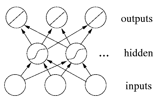
multi-layer network   (Fig. 1)

In principle, backprop provides a way to train networks with any number of hidden units arranged in any number of layers. (There are clear practical limits, which we will discuss later.) In fact, the network does not have to be organized in layers - any pattern of connectivity that permits a partial ordering of the nodes from input to output is allowed. In other words, there must be a way to order the units such that all connections go from "earlier" (closer to the input) to "later" ones (closer to the output). This is equivalent to stating that their connection pattern must not contain any cycles. Networks that respect this constraint are called feedforward networks; their connection pattern forms a directed acyclic graph or dag.


The Algorithm

We want to train a multi-layer feedforward network by gradient descent to approximate an unknown function, based on some training data consisting of pairs (x,t). The vector x represents a pattern of input to the network, and the vector t the corresponding target (desired output). As we have seen before, the overall gradient with respect to the entire training set is just the sum of the gradients for each pattern; in what follows we will therefore describe how to compute the gradient for just a single training pattern. As before, we will number the units, and denote the weight from unit j to unit i by wij.

  1. Definitions:
    • the error signal for unit j:
    delta_j = - partial E/partial net_j
    • the (negative) gradient for weight wij:
    Delta w_{ij} = -partial E/partial w_ij  
    • the set of nodes anterior to unit i:
    A_i = {j : exists w_ij}  
    • the set of nodes posterior to unit j:
    P_j = {i : exists w_ij}  

  2. The gradient. As we did for linear networks before, we expand the gradient into two factors by use of the chain rule:

    Delta w_ij = -(partial E/partial net_i) (partial net_i/partial w_ij)
    The first factor is the error of unit i. The second is

    partial net_i/partial w_ij =
(partial/partial w_ij) sum_{k in A_i} y_i w_ik = y_j
    Putting the two together, we get
    Delta w_ij = delta_i y_j.

    To compute this gradient, we thus need to know the activity and the error for all relevant nodes in the network.

  3. Forward activaction. The activity of the input units is determined by the network's external input x. For all other units, the activity is propagated forward:

    y_i = f_i(sum_{j in A_i} w_ij y_j)

    Note that before the activity of unit i can be calculated, the activity of all its anterior nodes (forming the set Ai) must be known. Since feedforward networks do not contain cycles, there is an ordering of nodes from input to output that respects this condition.

  4. Calculating output error. Assuming that we are using the sum-squared loss

    E = 1/2 sum_o (t_o - y_o)^2
    the error for output unit o is simply
    delta_o = t_o - y_o

  5. Error backpropagation. For hidden units, we must propagate the error back from the output nodes (hence the name of the algorithm). Again using the chain rule, we can expand the error of a hidden unit in terms of its posterior nodes:

    delta_j = -sum_{i in P_j} (partial E/partial net_i)
 (partial net_i/partial y_j) (partial y_j/partial net_j)

    Of the three factors inside the sum, the first is just the error of node i. The second is

    partial net_i/partial y_j = (partial/partial y_j)
 sum_{k in A_i} w_ik y_k = w_ij

    while the third is the derivative of node j's activation function:

    partial y_j/partial net_j =
 partial f_j(net_j)/partial net_j = f'_j(net_j)

    For hidden units h that use the tanh activation function, we can make use of the special identity
    tanh(u)' = 1 - tanh(u)2, giving us

    f'_h(net_h) = 1 - y_h^2

    Putting all the pieces together we get

    delta_j = f'_j(net_j) sum_{i in P_j} delta_i w_{ij}

    Note that in order to calculate the error for unit j, we must first know the error of all its posterior nodes (forming the set Pj). Again, as long as there are no cycles in the network, there is an ordering of nodes from the output back to the input that respects this condition. For example, we can simply use the reverse of the order in which activity was propagated forward.


Matrix Form

For layered feedforward networks that are fully connected - that is, each node in a given layer connects to every node in the next layer - it is often more convenient to write the backprop algorithm in matrix notation rather than using more general graph form given above. In this notation, the biases weights, net inputs, activations, and error signals for all units in a layer are combined into vectors, while all the non-bias weights from one layer to the next form a matrix W. Layers are numbered from 0 (the input layer) to L (the output layer). The backprop algorithm then looks as follows:

  1. Initialize the input layer:
    vec{y}_0 = vec{x}

  2. Propagate activity forward: for l = 1, 2, ..., L,
    vec{y}_l = f_l(W_l vec{y}_{l-1} + vec{b}_l)
    where bl is the vector of bias weights.

  3. Calculate the error in the output layer:
    vec{delta}_L = vec{t} - vec{y}_L

  4. Backpropagate the error: for l = L-1, L-2, ..., 1,
    vec{delta}_l = (W_{l+1}^T vec{delta}_{l+1}) . f'_l(vec{net}_l)
    where T is the matrix transposition operator.

  5. Update the weights and biases:
    Delta W_l = vec{delta}_l vec{y}_{l-1}^T, Delta vec{b}_l = vec{delta}_l

You can see that this notation is significantly more compact than the graph form, even though it describes exactly the same sequence of operations.


[Top] [Next: A first example] [Back to the first page]